Excel LAMBDA · Free to use, free to modify
Time Series and Statistical LAMBDAs
Simulated paths with fits to history, seasonal ARIMA forecasts with a band, fan charts, and the diagnostics that check the inputs first, as native Excel LAMBDA functions.
- LAMBDA
- Time series
- Forecasting
- Statistics
Detail
A single number for next year's revenue hides the question that matters: how wide is the range around it, and how does that range grow month by month? Answering it in Excel has usually meant an add-in or a second language, and the same is true of the statistical checks that should come before any model is trusted: are these inputs correlated, are they normal, is one of them an outlier?
This is a library of 54 LAMBDA functions that does that work natively. Seven simulators — geometric Brownian motion, jump-diffusion, two mean-reverting processes, ARMA, ARIMA and GARCH — each spill a block of paths, one row per trial and one column per period, and each has a Fit function that estimates its parameters from a history. Seasonal ARIMA fits a monthly or quarterly series, forecasts it with a band, simulates it, backtests it and ranks candidate models. A fan chart turns any block of paths into its P10 to P90 band over time. Six diagnostics check a table of data for correlation, normality, multicollinearity and outliers, each in a single spill whose size you know in advance.
The results do not move. Randomness comes from the same HDR generator as the Monte Carlo library: each number is a fixed function of the trial, the period, the series' VarID and a seed. Nothing is volatile, so a model recalculates only when its inputs change, and the same model gives the same answer on every machine. Give every simulated series its own VarID and change the seed for a fresh, equally repeatable draw.
The library is published as a public gist (https://gist.github.com/wfphillips128/96171c91caba82aa708b12b9f8f575ce (opens in a new tab)) that can be imported with any LAMBDA manager that reads gists. It is self-contained: the few building blocks it shares with the Monte Carlo library are included, character for character identical, so the two gists install safely into one workbook in either order. The functions become defined names inside the workbook and travel with the file. It needs Microsoft 365 or Excel 2024.
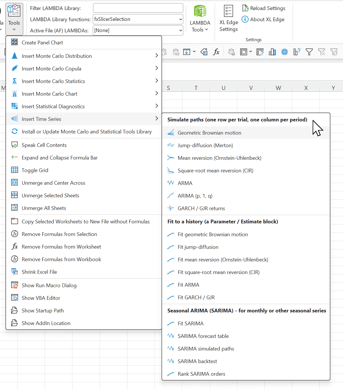
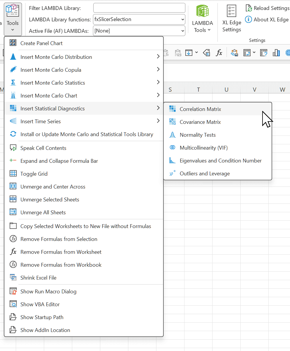
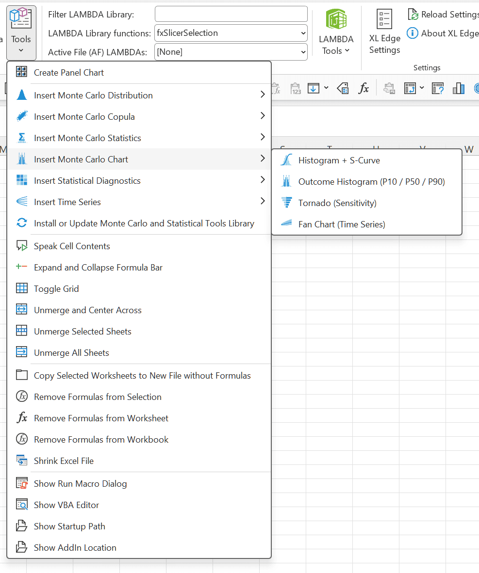
XL Edge needs no gist at all: it carries its own copy and installs only the functions each action uses. Two fly-outs on its Tools menu write the formulas. Insert Time Series prompts for a simulator's parameters, a fit's history or a SARIMA step, and checks there is room for the spill before writing. Insert Statistical Diagnostics writes any of the six checks for a selected table. The Chart fly-out adds a Fan Chart that draws a native Excel chart from any block of paths, with an optional plan line against the band.
Simulating paths
Every simulator spills Trials rows by Periods columns. Summarise any period like any other column of trials — =fx.RiskStatsλ(TAKE(B2#, , -1)) for the last one — or hand the whole block to the fan chart.
dt is the length of one period in the units of the rates: annual drift and volatility with monthly steps is dt = 1/12. DegFree swaps the normal shocks for Student t shocks scaled to the same variance — fat tails without changing the volatility. Start for ARMA is the values before period 1, oldest first; for ARIMA it is the last observed level. An ARMA whose AR part is not stationary returns #NUM!: use ARIMA for a series that trends.
Trials may also be a Trials × Periods block of uniforms — bootstrapped or correlated — which is then used as the shocks. And =100 * EXP(fx.RiskCumulateλ(D2#)) turns a block of log returns into prices.
| Function | Arguments | What it models |
|---|---|---|
| fx.RiskGBMλ=fx.RiskGBMλ(100, 0.08, 0.25, 12, 1/12, [Trials], [VarID], [Seed]) | Start, Drift, Volatility, Periods, [dt], [Trials], [VarID], [Seed] | Geometric Brownian motion: prices whose log changes are normal, growing at a steady rate with proportional noise. E[S(t)] = Start · e^(Drift · t). Returns periods 1 onwards; Start itself is not included. |
| fx.RiskJumpDiffusionλ=fx.RiskJumpDiffusionλ(100, 0.08, 0.2, 1, -0.1, 0.05, 12, 1/12, [Trials], [VarID], [Seed]) | Start, Drift, Volatility, JumpRate, JumpMean, JumpStDev, Periods, [dt], [Trials], [VarID], [Seed] | Merton's jump-diffusion: GBM plus sudden jumps arriving at JumpRate, each multiplying the price by e^N(JumpMean, JumpStDev). The drift is compensated, so jumps add risk without changing the expected path. A negative JumpMean models crashes. |
| fx.RiskOUλ=fx.RiskOUλ(0.04, 0.05, 0.8, 0.01, 60, 1/12, [DegFree], [Trials], [VarID], [Seed]) | Start, LongRunMean, Speed, Volatility, Periods, [dt], [DegFree], [Trials], [VarID], [Seed] | Ornstein–Uhlenbeck mean reversion: a value pulled back towards its long-run mean, such as a rate, a spread or a loss ratio. Exact discretisation; half-life = LN(2) / Speed. |
| fx.RiskCIRλ=fx.RiskCIRλ(0.04, 0.05, 0.8, 0.05, 60, 1/12, [Trials], [VarID], [Seed]) | Start, LongRunMean, Speed, Volatility, Periods, [dt], [Trials], [VarID], [Seed] | Cox–Ingersoll–Ross square-root mean reversion: like Ornstein–Uhlenbeck, but the noise shrinks towards zero, so the value never goes negative. Simulated with Andersen's quadratic-exponential scheme, which reproduces the exact mean and variance of every step. |
| fx.RiskARMAλ=fx.RiskARMAλ({0.6;0.2}, 0, 50, 4, 36, [Start], [DegFree], [Trials], [VarID], [Seed]) | AR, MA, Mean, StDev, Periods, [Start], [DegFree], [Trials], [VarID], [Seed] | ARMA(p, q) around a mean: each value leans on the ones before it (AR) and on recent shocks (MA). AR(p) alone is MA = 0. |
| fx.RiskARIMAλ=fx.RiskARIMAλ(0.3, 0, 0.5, 2, 24, 100, [DegFree], [Trials], [VarID], [Seed]) | AR, MA, Drift, StDev, Periods, [Start], [DegFree], [Trials], [VarID], [Seed] | ARIMA(p, 1, q): the period-to-period changes follow an ARMA with mean Drift, so the level wanders rather than returning to a mean. |
| fx.RiskGARCHλ=fx.RiskGARCHλ(0, 0.00001, 0.08, 0.9, 250, 0.05, [StartVariance], [DegFree], [Trials], [VarID], [Seed]) | Mean, Omega, Alpha, Beta, Periods, [Gamma], [StartVariance], [DegFree], [Trials], [VarID], [Seed] | GARCH(1,1) returns with volatility clusters: calm and turbulent stretches. ARCH(1) is Beta = 0; a Gamma adds the GJR extra reaction to bad news. Needs Alpha + Beta + Gamma / 2 < 1. |
Every simulator ends with [Trials] (default 10,000, or a block of uniforms to use as the shocks), [VarID] (default 1) and [Seed] (default 0). An argument still in [brackets] is optional and can be left out. Speed, at 10,000 trials: 60 periods take 0.5 to 1.8 seconds per model, 250 periods 3.4 to 7 seconds.
Fitting to a history
Each fit returns a Parameter / Estimate block. Point the simulator's arguments at its cells and the paths are calibrated to the history, and recalibrate themselves when the history is extended.
For ARIMA, fit the changes: =fx.RiskFitARMAλ(DROP(A2:A500, 1) - DROP(A2:A500, -1), 1, 1), and its Mean is the Drift. On simulated histories every fit recovers the true parameters. The ARMA fit lands within 0.05 of an independent maximum-likelihood implementation and the GARCH fit within 0.01. The jump-diffusion fit leans on sixth moments, which need thousands of observations: treat it as a first guess.
| Function | Arguments | Block | Method |
|---|---|---|---|
| fx.RiskFitGBMλ=fx.RiskFitGBMλ(B2:B61, 1/12) | Prices, [dt] | 3 × 2 | The mean and standard deviation of the log returns. Exact. |
| fx.RiskFitJumpDiffusionλ=fx.RiskFitJumpDiffusionλ(B2:B2501, 1/252) | Prices, [dt] | 6 × 2 | The 2nd, 4th and 6th cumulants of the log returns, assuming symmetric jumps (after Press, 1967). A rough starting point. |
| fx.RiskFitOUλ=fx.RiskFitOUλ(C2:C121, 1/12) | Series, [dt] | 5 × 2 | Least squares of each value on the one before. Exact for the exact discretisation; adds the half-life. |
| fx.RiskFitCIRλ=fx.RiskFitCIRλ(C2:C121, 1/12) | Series, [dt] | 4 × 2 | Least squares on square-root-scaled changes. The Euler form, so approximate. |
| fx.RiskFitARMAλ=fx.RiskFitARMAλ(D2:D200, 2, [MALags]) | Series, ARLags, [MALags] | (3 + p + q) × 2 | Conditional least squares for AR terms; Hannan–Rissanen when there are MA terms. |
| fx.RiskFitGARCHλ=fx.RiskFitGARCHλ(E2:E1001, TRUE) | Returns, [Asymmetric] | 7 × 2, or 8 with Gamma | Quasi maximum likelihood with variance targeting, on a grid refined twice (about ±0.001 fine). Asymmetric = TRUE fits GJR. |
Seasonal ARIMA (SARIMA)
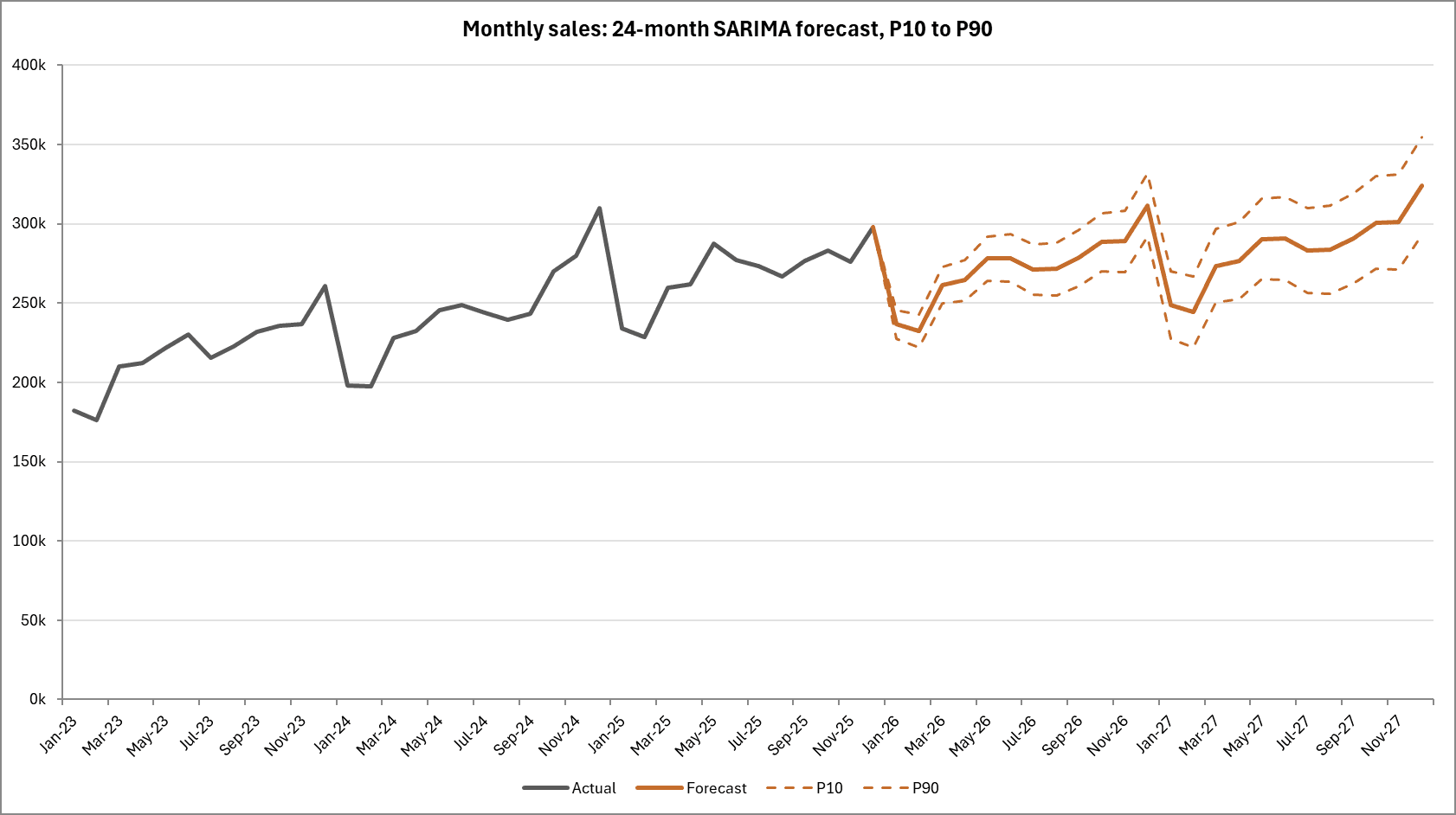
For monthly, weekly or quarterly series with a repeating seasonal pattern: sales, policy counts, call volumes, claims. Five functions are built around a Model block. Fit writes it; Forecast and the simulator read it; Backtest and Rank refit by themselves. A worked sequence on 108 months of history in C4:C111: =fx.RiskSARIMAFitλ(C4:C111) in F2, then =fx.RiskSARIMAForecastλ(C4:C111, F2#, 24) for the next 24 months with a P10 to P90 band, =fx.RiskSARIMABacktestλ(C4:C111, 12) to ask how well last year would have been forecast, =fx.RiskSARIMARankλ(C4:C111) to compare candidate models, and =fx.RiskSARIMAλ(C4:C111, F2#, 24) for 10,000 simulated continuations to feed the fan chart.
Order is {p, d, q, P, D, Q}, up to p, q = 2, P, Q = 1 and d, D = 1. The default is the classic airline model {0,1,1,0,1,1}, a good first choice for business series. Log = TRUE models the logarithm: seasonal swings that grow with the level, a forecast that cannot go negative, and a band wider above than below. The Model block can also be typed by hand, with parameters estimated elsewhere.
The forecast band is exact for the model — the forecast ± z × StDev × √Σψ² — so the percentiles of the simulated paths match the table. Backtest Coverage is how often the actuals fell inside the band: near 80% is right for P10 to P90. Rank fits 12 common orders with the same differencing and compares their AIC on the same residual window; it is a guide, not a verdict, so backtest the leaders. On short series the coefficients are loosely determined by any method while the forecasts agree closely: judge a model by its forecasts and backtests, not by a single coefficient.
| Function | Arguments | Returns |
|---|---|---|
| fx.RiskSARIMAFitλ=fx.RiskSARIMAFitλ(C4:C111, [Order], [Season], [Log]) | History, [Order], [Season], [Log] | The Model block, 19 × 2: p, d, q, P, D, Q, Season, Log, Constant, AR1, AR2, MA1, MA2, SAR1, SMA1, StDev, AIC and Observations. Conditional sum of squares, minimised from a coarse grid by Levenberg–Marquardt. |
| fx.RiskSARIMAForecastλ=fx.RiskSARIMAForecastλ(C4:C111, F2#, 24, [Lower], [Upper], [Labels]) | History, Model, Horizon, [Lower], [Upper], [Labels] | (Horizon + 1) × 4: Period, Forecast and the band, P10 and P90 by default. |
| fx.RiskSARIMAλ=fx.RiskSARIMAλ(C4:C111, F2#, 24, [DegFree], [Trials], [VarID], [Seed]) | History, Model, Periods, [DegFree], [Trials], [VarID], [Seed] | Trials × Periods simulated continuations of the history, ready for the fan chart. |
| fx.RiskSARIMABacktestλ=fx.RiskSARIMABacktestλ(C4:C111, 12, [Order], [Season], [Log], [Lower], [Upper]) | History, Holdout, [Order], [Season], [Log], [Lower], [Upper] | (Holdout + 6) × 6: MAPE, RMSE, MAE, Bias and Coverage, then Period, Actual, Forecast, Error and the band for each held-out period. Refits without the last Holdout values. |
| fx.RiskSARIMARankλ=fx.RiskSARIMARankλ(C4:C111, [Diff], [SeasonalDiff], [Season], [Log]) | History, [Diff], [SeasonalDiff], [Season], [Log] | 13 × 3: twelve common orders ranked by AIC. |
A fit on 108 months takes well under a second, and Rank about a second. The fitted optimum matches an independent optimiser of the same objective to within 0.0001, and on 600 simulated months it agrees with an exact maximum-likelihood fit to 0.01.
Fan chart
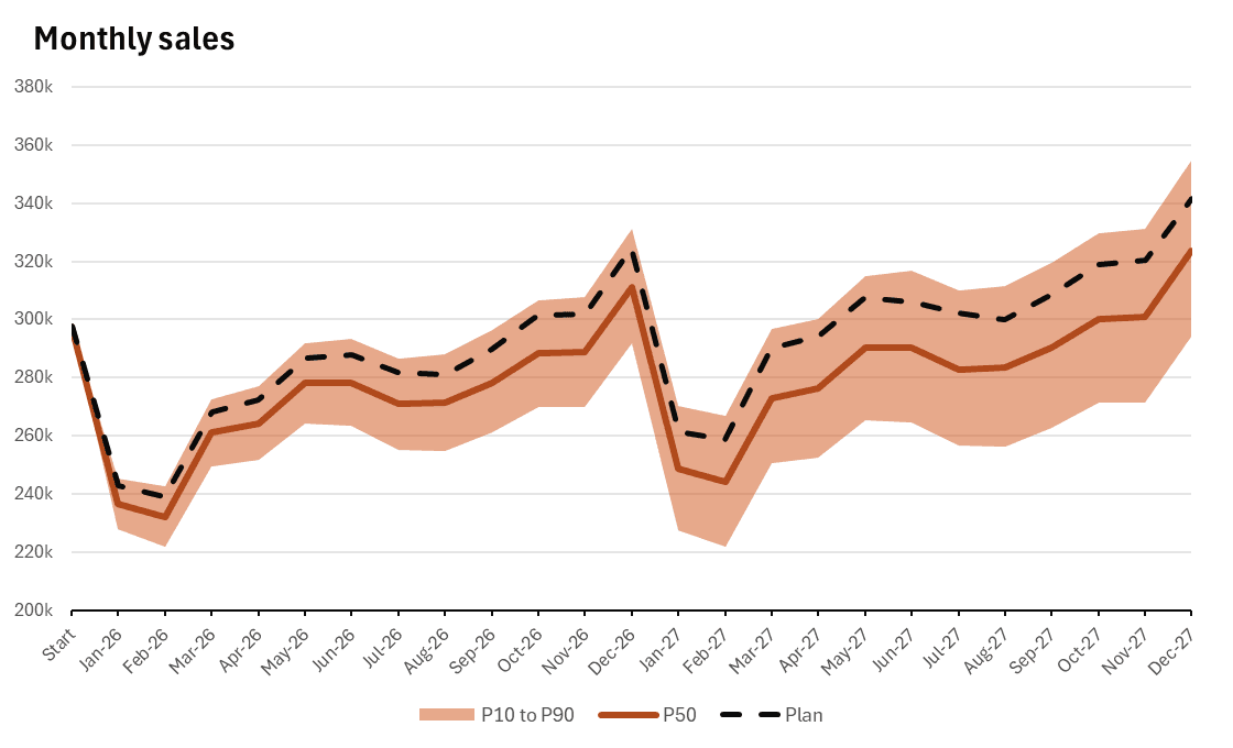
fx.RiskChartFanλ reads any block of paths — from a simulator, from SARIMA, or from a model built on them — and returns everything a fan chart needs in one spill: a title row, a header row, then one row per period with the lower percentile, P50, the upper percentile, the band's width, the plan and the mean. The band defaults to P10 to P90 and can be any pair; the headers are formulas, so a chart legend linked to them follows any change.
Plan is the single-number forecast the business already has, drawn as a line against the band — the picture of how likely the plan is. Start opens the fan from a point at period 0, and Labels puts dates on the axis. XL Edge's Insert Monte Carlo Chart → Fan Chart writes the data and draws the chart, and it redraws when the model changes.
| Function | Arguments | Returns |
|---|---|---|
| fx.RiskChartFanλ=fx.RiskChartFanλ(H2#, [Lower], [Upper], A1, [Start], C2:C13, B2:B13) | Paths, [Lower], [Upper], [Name], [Start], [Plan], [Labels] | (Periods + 2) × 7, one more row with Start: the title, the headers, then Period, Lower, P50, Upper, band width, Plan and Mean for each period. |
Statistical diagnostics
Checks on a table of history, one variable per column, or on simulated inputs side by side with HSTACK(B2#, C2#, D2#). Each returns one labelled spill whose size is known in advance, so XL Edge can check there is room before writing it.
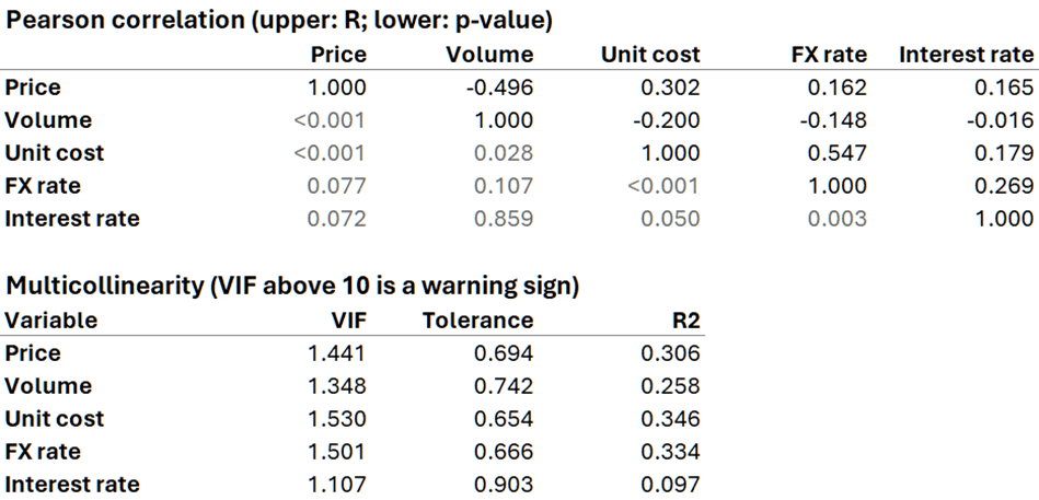
Correlation is Pearson, or Spearman on ranks. The upper triangle always shows R; LowerTriangle puts something else below it: 0 only the strong pairs (|R| > 0.90), 1 R squared, 2 p-values, 3 Yes / No for significance at Alpha. Labels = FALSE returns the bare matrix, ready for fx.RiskCopulaGaussλ on the Monte Carlo LAMBDAs page — a copula fitted from history in two formulas.
Normality runs Shapiro–Wilk, Anderson–Darling and Jarque–Bera, each with its p-value and a verdict at Alpha (default 0.05). Be careful with thousands of values: every test then rejects even trivial departures from normality. These tests earn their keep on histories and on model residuals. Multicollinearity reports the VIF — how much a variable's variance is inflated because the others explain it — with Tolerance and R²; above 10 is a warning sign. The eigenvalues come with the condition number, where above 30 signals serious multicollinearity. Outliers gives every row its Mahalanobis distance from the centre and its leverage, each with a flag.
| Function | Arguments | Returns |
|---|---|---|
| fx.RiskCorrelMatrixλ=fx.RiskCorrelMatrixλ(B2:F200, 2, [Method], [Alpha], [Names], [Labels]) | Data, [LowerTriangle], [Method], [Alpha], [Names], [Labels] | (k + 2) × (k + 1): the correlation matrix with names, and the chosen measure below the diagonal. k × k with Labels = FALSE. |
| fx.RiskCovMatrixλ=fx.RiskCovMatrixλ(B2:F200, [Sample], [Names], [Labels]) | Data, [Sample], [Names], [Labels] | (k + 2) × (k + 1): the covariance matrix, sample or population. k × k with Labels = FALSE. |
| fx.RiskNormalityλ=fx.RiskNormalityλ(B2:F200, [Tests], [ADVariant], [Alpha], [Names]) | Data, [Tests], [ADVariant], [Alpha], [Names] | 14 × (k + 1): each test's statistic, p-value and verdict for every variable. ADVariant is "Normal" (the usual), "Unmodified", "LogNormal" or "Generic" for data already standardised, such as residuals. |
| fx.RiskCollinearityλ=fx.RiskCollinearityλ(B2:F200, "All", [Names]) | Data, [Measure], [Names] | (k + 2) × 2, or × 4 with "All": VIF, Tolerance (1 / VIF) and R² for each variable. |
| fx.RiskEigenλ=fx.RiskEigenλ(B2:F200) | Data | (k + 2) × 5: the eigenvalues of the correlation matrix, largest first, with the condition number. Data may also be a correlation matrix. |
| fx.RiskOutliersλ=fx.RiskOutliersλ(B2:F200) | Data | (n + 2) × 5: each row's Mahalanobis distance, flagged above the mean distance plus one standard deviation, and its leverage, flagged above 2(k + 1) / n. |
k is the number of variables (columns) and n the number of rows. Excel has no eigenvalue function, so the eigenvalues come from a Jacobi solver, fx.RiskJacobiλ, exact for up to about 30 variables. Shapiro–Wilk uses Royston's algorithm and accepts 3 to 5,000 values.
Building blocks
The functions above are built on these. They are ordinary functions and can be called from a sheet, but most models will never need to.
| Function | Arguments | Returns |
|---|---|---|
| fx.RiskTSUλ | Trials, Periods, VarID, Seed, [Stream] | The Trials × Periods block of uniforms behind every simulator, on its own HDR stream so a path never shares one with a distribution or a copula. |
| fx.RiskTSShocksλ | U, [DegFree] | Standardised shocks from those uniforms: normal, or Student t scaled to unit variance. |
| fx.RiskTSRecurseλ | Inputs, Start, NextValue | A one-number recursion run along every row with a single SCAN — the engine of the ARMA, ARIMA and GARCH paths. |
| fx.RiskCumulateλ | Increments, [Start] | Running totals along each row: levels from changes, or log prices from log returns. |
| fx.RiskARStationaryλ | AR | TRUE when the AR coefficients are stationary, by the Durbin–Levinson step-down to partial autocorrelations. |
| fx.RiskTSImpulseλ | AR, MA, Periods | The ARMA impulse-response (ψ-weight) matrix. |
| fx.RiskLagMatrixλ | X, Lags | A matrix of lagged copies of a series, for the ARMA fit. |
| fx.RiskGARCHLogLikλ | Resid, TargetVar, Alpha, Beta, Gamma | The GARCH log-likelihood the fit maximises. |
| fx.RiskDifferenceλ | X, Diff, SeasonalDiff, Season | Differences a series, ordinarily and seasonally. |
| fx.RiskPolyMulλ | A, B | Multiplies two lag polynomials. |
| fx.RiskSARIMAPolyλ | Coefs, Season, Side | The multiplicative seasonal AR or MA polynomial. |
| fx.RiskSARIMASSEλ | W, Coefs, Season, Start | The conditional sum of squares SARIMA minimises, vectorised over sets of coefficients. |
| fx.RiskSARIMAResidλ | W, Coefs, Season, Start | The residuals for one set of coefficients; fx.RiskSARIMAResidsλ, with the same arguments, for many at once. |
| fx.RiskSARIMAMeanλ | History, Model, Periods | The SARIMA point forecast. |
| fx.RiskSARIMAImpulseλ | Model, Periods | The SARIMA impulse-response matrix behind the band and the paths. |
| fx.RiskCorrelλ | Data, [Method] | The bare correlation matrix, Pearson or Spearman. |
| fx.RiskShapiroWilkλ | X | One column's Shapiro–Wilk statistic and p-value. |
| fx.RiskAndersonDarlingλ | X, [Variant] | One column's Anderson–Darling statistic and p-value. |
| fx.RiskJarqueBeraλ | X | One column's Jarque–Bera statistic and p-value. |
| fx.RiskJacobiλ | Matrix, [Sweeps] | The eigenvalues of a symmetric matrix, largest first, by Jacobi rotations. |
Eight more come from the Monte Carlo library and are included so this gist installs on its own: fx.RiskHDRλ, fx.RiskUλ, fx.RiskPoissonλ (the jump counts), fx.RiskDiscreteInvλ, fx.RiskHalfTInvλ, fx.RiskVarNameλ, fx.RiskVarNamesλ and fx.RiskRankλ. They are documented on the Monte Carlo LAMBDAs page.
Conventions worth checking
These get a wrong answer rather than an error, so they are stated plainly.
- dt is in the units of the rates. Annual drift and volatility with monthly periods is dt = 1/12. Leave it out and every period is one whole unit — a year of growth per month.
- ARMA and ARIMA read Start differently. For ARMA it is the values before period 1, oldest first, and defaults to the mean. For ARIMA it is the last observed level, and defaults to 0.
- GARCH needs Alpha + Beta + Gamma / 2 < 1. Otherwise the variance has no long-run level. The fit enforces it; a hand-typed set of parameters should be checked.
- Give every series its own VarID. Two series sharing a VarID draw identical shocks and move in lockstep. XL Edge's selector assigns a fresh one each time.
- Normality tests on thousands of values reject everything. With enough data any departure from normality is significant. Test histories and residuals, not 10,000 simulated trials.
- Judge SARIMA by its forecasts, not its coefficients. On a few years of monthly data different methods give different coefficients and nearly the same forecast. Backtest before choosing.
How it is checked
140 of the 557 automated checks that drive Excel directly cover this library, and all pass. Every simulator matches an independent step-by-step recursion cell for cell, to about 10⁻¹⁵, with normal and with Student t shocks; simulated means and variances match their closed forms; and a block of uniforms passed as Trials is used as the shocks exactly. Every fit equals an independent replica of its own method, and lands close to an independent maximum-likelihood fit — within 0.011 for ARMA and 0.008 for GARCH and GJR on the test histories.
SARIMA's fit, forecast, simulated paths, backtest and rank each match an independent replica, the forecast exactly; the percentiles of the simulated paths match the forecast table's band; and the fitted optimum matches an independent optimiser of the same objective to within 0.0001. Every diagnostic matches independent references: correlation, covariance, eigenvalues and distances, Pearson and Spearman p-values, Shapiro–Wilk, Anderson–Darling, Jarque–Bera and VIF. The fan chart's percentiles and means match to 10⁻¹⁶.
The rest cover invalid arguments, each of which must return an error rather than a plausible wrong number; timing at 10,000 trials by 60 and by 250 periods; and a call counter showing that nothing recalculates unless its own inputs change. A further 32 checks install both public gists into blank workbooks, save, reopen and recalculate, and confirm that a function the two share gives the same trials whichever gist goes in second.
Attribution
Every method here is implemented independently from its original publication; no code was taken. The sources are credited here and inside the library itself.
- ProbabilityManagement.org and Hubbard Decision Research (opens in a new tab) The HDR counter-based generator, published openly as part of the SIPmath standard; ChanceCalc Plus and PM_Lambda_functions, MIT licence, Copyright 2012–2026 Probability Management, Inc.
- ARMA, ARIMA and seasonal ARIMA Box, Jenkins and Reinsel, Time Series Analysis: Forecasting and Control (the multiplicative seasonal and airline models, ψ-weights); Hamilton, Time Series Analysis (1994); Hannan and Rissanen (Biometrika 69(1), 1982) for estimation with MA terms; Levenberg (1944) and Marquardt (1963) for the SARIMA minimisation.
- Continuous-time processes Glasserman, Monte Carlo Methods in Financial Engineering (2003); Merton (Journal of Financial Economics 3, 1976) for jump-diffusion and Press (Journal of Business 40(3), 1967) for its cumulant fit; Vasicek (1977); Cox, Ingersoll and Ross (Econometrica 53(2), 1985), simulated with Andersen's quadratic-exponential scheme (Journal of Computational Finance 11(3), 2008).
- GARCH and GJR Engle (1982); Bollerslev (Journal of Econometrics 31, 1986, and the scaled Student t shocks of 1987); Glosten, Jagannathan and Runkle (Journal of Finance 48(5), 1993); variance targeting after Engle and Mezrich (1996).
- Diagnostics Shapiro–Wilk by Royston's algorithm (Applied Statistics 44(4), 1995); Anderson–Darling after D'Agostino and Stephens, Goodness-of-Fit Techniques (1986), and Marsaglia and Marsaglia (Journal of Statistical Software 9(2), 2004); Jarque and Bera (International Statistical Review 55(2), 1987); VIF, condition number and leverage after Belsley, Kuh and Welsch, Regression Diagnostics (1980); Mahalanobis (1936); the Jacobi eigenvalue method after Golub and Van Loan, Matrix Computations.