Excel LAMBDA · Free to use, free to modify
Distribution LAMBDAs for Monte Carlo Simulations
Thirty-nine Monte Carlo distributions, five copulas for correlated inputs, risk measures and chart data as native Excel LAMBDA functions. Each one spills every trial from a single cell, gives the same answer on every recalculation, and needs no legacy or expensive Monte Carlo add-in to open.
- LAMBDA
- Monte Carlo
- Dynamic arrays
- Statistics
Detail
Monte Carlo simulation in Excel has usually meant an add-in: XLRisk, @RISK, Argo, and others. Most of them pre-date modern Excel. They are not being updated to take advantage of dynamic arrays or LAMBDA, and every person who opens the model needs the same add-in installed, or the inputs turn into errors.
This is a library of 79 LAMBDA functions that does the same job natively: 39 distributions, five copulas that make inputs move together, the statistics, risk measures and chart data that read the results, and the building blocks underneath. Each distribution spills all of its trials from a single cell — =fx.RiskPertλ(80, 100, 150, 10000, 1) returns 10,000 samples of a three-point cost estimate — so the model itself is ordinary array arithmetic. Multiply two spilled ranges and every trial is calculated at once, with no simulation loop, no macro and no data table.
The results do not move. Randomness comes from the HDR generator, a counter-based formula in which each number is a fixed function of the trial number, the input's VarID and a seed. The functions are non-volatile: the same model gives the same answer on every machine, and neither editing an unrelated cell nor a full recalculation reshuffles the trials. Change the seed for a fresh, equally repeatable draw. RAND is still available for live resampling, and Latin hypercube sampling is one argument away.
The library is published as a single public gist (https://gist.github.com/wfphillips128/f91bff77212ab2c3d8f55a4f0a51b8b6 (opens in a new tab)) which can be imported with any LAMBDA manager that reads gists. The functions become defined names inside the workbook, so they travel with the file: anyone you send it to can open it and it calculates. It needs Microsoft 365 or Excel 2024. To update, re-import the gist — and try the first import in a blank workbook, because importing replaces any existing name that matches.
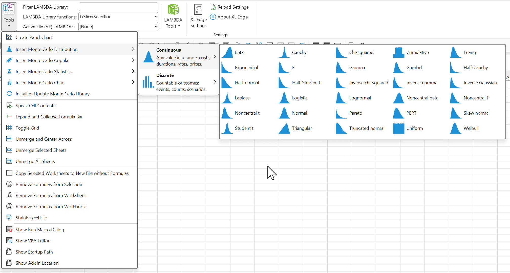
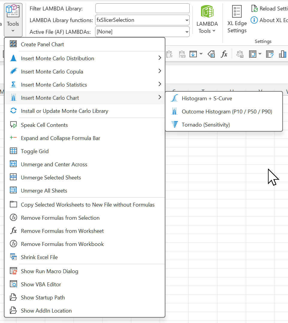
XL Edge makes the functions quicker to use, and needs no gist at all: it carries its own copy of the library and installs only the functions each action uses, plus whatever they depend on, so a workbook holds what its model needs and nothing more. Its Tools menu inserts a distribution from a selector: it prompts for each parameter and writes a native formula such as =fx.RiskPertλ($C$4, $C$5, $C$6, MC_Trials, 7), with the trial count held in one workbook name and a fresh VarID assigned to every input. Three more fly-outs insert a copula, the statistics — a summary or detailed block for one result, a table for several, histogram data and the risk measures — and a finished Excel chart: a histogram with its S-curve, an outcome histogram marked at P10, P50 and P90, or a tornado of which inputs move the result most.
Continuous distributions
Every distribution is an inverse-CDF transform of one uniform stream, u, from fx.RiskUλ. None uses rejection sampling or a loop, which is what lets each one be a single spilling formula. Argument order follows XLRisk and @RISK, so an existing model migrates by name.
Twenty-five of the thirty have a closed form or are built on Excel's own GAMMA.INV, BETA.INV and NORM.S.INV. The other five — the inverse Gaussian, the skew normal and the three noncentral distributions — have no inverse in Excel, so they are sampled by numeric inversion: the CDF is evaluated once on a 4,096-point grid and every trial is interpolated from it. That is accurate to about 10⁻⁸ relative, and 100,000 trials take about a second.
Degrees of freedom may be fractional. Excel's own CHISQ.INV, T.INV and F.INV silently truncate them to whole numbers, which is why none of them is used.
| Function | Arguments | How it samples |
|---|---|---|
| fx.RiskBetaλ=fx.RiskBetaλ(5, 2, [A], [B], [Trials], [VarID], [Seed]) | Shape1, Shape2, [A], [B] | BETA.INV on the two shape parameters, rescaled to the range A to B (default 0 to 1). |
| fx.RiskCauchyλ=fx.RiskCauchyλ(0, 1, [Trials], [VarID], [Seed]) | Location, Scale | Location + Scale × TAN(π(u − ½)), switching to the cotangent form in the tails so precision holds near 0 and 1. Has no mean or variance — expect wild extremes. |
| fx.RiskChiSqλ=fx.RiskChiSqλ(3, [Trials], [VarID], [Seed]) | DegFree | GAMMA.INV(u, DegFree / 2, 2). |
| fx.RiskCumulλ=fx.RiskCumulλ(0, 100, {20,50,80}, {0.1,0.5,0.9}, [Trials], [VarID], [Seed]) | MinValue, MaxValue, XValues, YValues | Straight-line interpolation between points on the cumulative curve, anchored at 0 at MinValue and 1 at MaxValue. For percentile estimates. |
| fx.RiskErlangλ=fx.RiskErlangλ(4, 5, [Trials], [VarID], [Seed]) | K, Beta | GAMMA.INV with a whole-number shape K and scale Beta: the waiting time until the Kth event. |
| fx.RiskExponλ=fx.RiskExponλ(5, [Trials], [VarID], [Seed]) | Mean | −Mean × LN(1 − u). Takes the mean, not the rate. |
| fx.RiskExtValueλ=fx.RiskExtValueλ(0, 1, [Trials], [VarID], [Seed]) | Location, Scale | Location − Scale × LN(−LN(u)). The Gumbel distribution of maxima — floods, peak loads, worst days. @RISK's RiskExtValue. |
| fx.RiskFλ=fx.RiskFλ(5, 10, [Trials], [VarID], [Seed]) | NumDF, DenDF | (DenDF / NumDF) × X / (1 − X) with X beta-distributed. X and 1 − X each come from their own BETA.INV, so neither is formed as 1 minus a number near 1. |
| fx.RiskGammaλ=fx.RiskGammaλ(2, 1, [Trials], [VarID], [Seed]) | Alpha, Beta | GAMMA.INV with shape Alpha and scale Beta. |
| fx.RiskHalfCauchyλ=fx.RiskHalfCauchyλ(1, [Location], [Trials], [VarID], [Seed]) | Scale, [Location] | Location + Scale × TAN(πu / 2), with the cotangent form above the median. Location is the lower bound, default 0. |
| fx.RiskHalfNormalλ=fx.RiskHalfNormalλ(1, [Location], [Trials], [VarID], [Seed]) | Scale, [Location] | Location + Scale × √GAMMA.INV(u, ½, 2) — the size of a normal deviation, exact even for tiny u. |
| fx.RiskHalfStudentλ=fx.RiskHalfStudentλ(3, 1, [Location], [Trials], [VarID], [Seed]) | DegFree, Scale, [Location] | Location + Scale × the quantile of |t|, from a pair of BETA.INV calls (fx.RiskHalfTInvλ). |
| fx.RiskInvChiSqλ=fx.RiskInvChiSqλ(6, [Trials], [VarID], [Seed]) | DegFree | 1 / GAMMA.INV(1 − u, DegFree / 2, 2): the reciprocal of a chi-squared. |
| fx.RiskInvGammaλ=fx.RiskInvGammaλ(3, 2, [Trials], [VarID], [Seed]) | Alpha, Beta | Beta / GAMMA.INV(1 − u, Alpha, 1): the reciprocal of a gamma. @RISK's RiskPearson5. |
| fx.RiskInvGaussλ=fx.RiskInvGaussλ(1, 1.5, [Trials], [VarID], [Seed]) | Mean, Shape | Numeric inversion of the inverse Gaussian (Wald) CDF, combined in logs so it cannot overflow. The variance is Mean³ / Shape. |
| fx.RiskLaplaceλ=fx.RiskLaplaceλ(0, 1, [Trials], [VarID], [Seed]) | Location, Scale | Location + Scale × LN(2u) below the median, Location − Scale × LN(2(1 − u)) above it. A scale, not the sd: sd = Scale × √2. |
| fx.RiskLogisticλ=fx.RiskLogisticλ(0, 1, [Trials], [VarID], [Seed]) | Location, Scale | Location + Scale × LN(u / (1 − u)). A scale, not the sd: sd = Scale × π / √3. |
| fx.RiskLogNormλ=fx.RiskLogNormλ(0, 0.45, [Trials], [VarID], [Seed]) | Mean, StDev | LOGNORM.INV. Mean and StDev are those of ln(X), as in @RISK's RiskLognorm2. |
| fx.RiskNCBetaλ=fx.RiskNCBetaλ(2, 5, 6, [Trials], [VarID], [Seed]) | Shape1, Shape2, NonCentrality | Numeric inversion of the noncentral beta CDF, a Poisson-weighted sum of BETA.DIST terms. |
| fx.RiskNCFλ=fx.RiskNCFλ(5, 20, 8, [Trials], [VarID], [Seed]) | NumDF, DenDF, NonCentrality | Numeric inversion through the noncentral beta CDF, on the same grid. Power calculations for F tests. |
| fx.RiskNCStudentλ=fx.RiskNCStudentλ(6, 3, [Trials], [VarID], [Seed]) | DegFree, NonCentrality | Numeric inversion of the noncentral t CDF, using Lenth's series (AS 243). Power calculations for t tests. |
| fx.RiskNormalλ=fx.RiskNormalλ(100, 15, [Trials], [VarID], [Seed]) | Mean, StDev | NORM.INV. |
| fx.RiskParetoλ=fx.RiskParetoλ(2, 1, [Trials], [VarID], [Seed]) | Theta, A | A × (1 − u)^(−1 / Theta). Shape first, then the scale, which is the minimum possible value. |
| fx.RiskPertλ=fx.RiskPertλ(5, 10, 25, [Trials], [VarID], [Seed]) | Min, Mode, Max | BETA.INV with α = (4·Mode + Max − 5·Min) / (Max − Min) and β = (5·Max − Min − 4·Mode) / (Max − Min), scaled to Min to Max. A smoother three-point estimate than triangular. |
| fx.RiskSkewNormalλ=fx.RiskSkewNormalλ(0, 1, 6, [Trials], [VarID], [Seed]) | Location, Scale, Shape | Numeric inversion of Φ(z) − 2·T(z, Shape), using Owen's T function. Shape 0 gives the normal. |
| fx.RiskStudentλ=fx.RiskStudentλ(2, [Trials], [VarID], [Seed]) | DegFree | The sign of u − ½ times the quantile of |t| from two BETA.INV calls. The standard t, centred on 0: use Location + Scale × … to shift it. |
| fx.RiskTriangλ=fx.RiskTriangλ(5, 70, 95, [Trials], [VarID], [Seed]) | Min, Mode, Max | The closed-form two-branch quantile: Min + √(u·(Mode − Min)·(Max − Min)) below the mode, Max − √((1 − u)·(Max − Mode)·(Max − Min)) above it. |
| fx.RiskTruncNormalλ=fx.RiskTruncNormalλ(0, 1, -0.3, 2.5, [Trials], [VarID], [Seed]) | Mean, StDev, [Min], [Max] | NORM.S.INV of u rescaled into the window between the bounds, worked in whichever tail the window sits so a window far from the mean keeps its precision. Omit a bound for a one-sided truncation. |
| fx.RiskUniformλ=fx.RiskUniformλ(0, 1, [Trials], [VarID], [Seed]) | Min, Max | Min + u × (Max − Min). |
| fx.RiskWeibullλ=fx.RiskWeibullλ(2.5, 20, [Trials], [VarID], [Seed]) | Alpha, Beta | Beta × (−LN(1 − u))^(1 / Alpha). Shape first, then scale. |
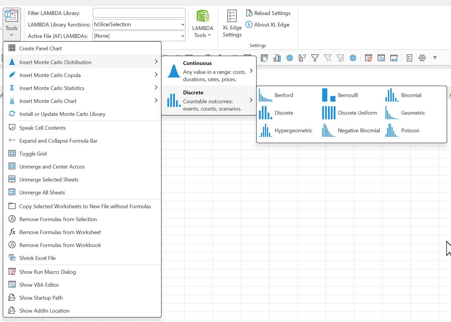
Every distribution, continuous and discrete, ends with the same three optional arguments: [Trials] (default 10,000, or an array of uniforms to use instead), [VarID] (default 1) and [Seed] (default 0). The example under each function name gives the shape pictured on that distribution's XL Edge icon; an argument still in [brackets] is optional and can be left out. Invalid arguments return #NUM! rather than a plausible-looking wrong number.
Discrete distributions
| Function | Arguments | How it samples |
|---|---|---|
| fx.RiskBenfordλ=fx.RiskBenfordλ(1, [Trials], [VarID], [Seed]) | [Digits] | The closed-form inverse of Benford's law, P(d) = LOG10(1 + 1/d), checked once against the CDF. First digits 1–9 by default; Digits = 2 gives the first two digits, 10–99, as used in forensic accounting tests. |
| fx.RiskBernoulliλ=fx.RiskBernoulliλ(0.3, [Trials], [VarID], [Seed]) | P | 1 when u > 1 − P, otherwise 0. Does the event happen? Identical to fx.RiskBinomialλ(1, P). |
| fx.RiskBinomialλ=fx.RiskBinomialλ(10, 0.2, [Trials], [VarID], [Seed]) | N, P | BINOM.INV(N, P, u): the number of successes in N independent tries. |
| fx.RiskDiscreteλ=fx.RiskDiscreteλ({1,2,3,4,5}, {0.2,0.3,0.3,0.15,0.05}, [Trials], [VarID], [Seed]) | Values, Probabilities | A running total of the probabilities with SCAN, then an XLOOKUP of u against it. The probabilities must sum to 1. |
| fx.RiskDUniformλ=fx.RiskDUniformλ({1,2,3,4,5}, [Trials], [VarID], [Seed]) | Values | INDEX(Values, INT(u × n) + 1): every value in the list equally likely. |
| fx.RiskGeometλ=fx.RiskGeometλ(0.35, [Trials], [VarID], [Seed]) | P | CEILING(LN(1 − u) / LN(1 − P)) − 1, checked once against the CDF. Counts failures before the first success, from 0. |
| fx.RiskHypergeoλ=fx.RiskHypergeoλ(10, 12, 30, [Trials], [VarID], [Seed]) | Draws, Successes, Population | A binary search of u in a table of HYPGEOM.DIST over every possible count. Sampling without replacement — audit samples. @RISK's (n, D, M). |
| fx.RiskNegbinλ=fx.RiskNegbinλ(3, 0.5, [Trials], [VarID], [Seed]) | Successes, P | A binary search of u in a CDF table built with BETA.DIST — not NEGBINOM.DIST, which truncates Successes to a whole number. Counts failures before the last success. |
| fx.RiskPoissonλ=fx.RiskPoissonλ(3, [Trials], [VarID], [Seed]) | Mean | A binary search of u in a table of POISSON.DIST wide enough to cover every count that can plausibly occur. Events in a fixed interval — claims, arrivals, defects. |
Copulas: inputs that move together
A distribution describes one input. A copula describes how several inputs move together. Price and volume, claim frequency and severity, interest rates and defaults are rarely independent, and a model that samples them as if they were understates how often the bad cases arrive at the same time.
Each copula spills a block of correlated uniforms, one column per input. Feed one column into each distribution's Trials argument and every input keeps exactly the distribution you gave it, while moving with the others: =fx.RiskCopulaGaussλ({1,0.7;0.7,1}, 10000, 20) in C2, then =fx.RiskNormalλ(100, 15, CHOOSECOLS(C2#, 1)) and =fx.RiskLogNormλ(0.5, 0.4, CHOOSECOLS(C2#, 2)). The copula owns the randomness, so give it its own VarID; the distributions fed from it take none. Its streams never collide with theirs.
The choice is about the tails. The Gaussian copula is the standard, symmetric choice, with no extra tendency for extremes to coincide. The Student t adds that tendency in both tails: fewer degrees of freedom, stronger. Clayton concentrates dependence in the lower tail — inputs that crash together — and Gumbel in the upper tail — inputs that boom together. Frank is symmetric with lighter tails than the Gaussian.
For two inputs, Clayton and Frank also take a negative Theta, so the inputs move in opposite directions: price up, volume down. The three Archimedean copulas — Clayton, Gumbel and Frank — take an optional Rotation, as in the VineCopula R package: 180 moves the tail to the other corner, and 90 or 270 turns positive dependence negative. XL Edge's Insert Monte Carlo Copula prompts for the correlation matrix or Theta, writes the block, and shows the formula to feed each column into a distribution.

| Function | Arguments | How it samples |
|---|---|---|
| fx.RiskCopulaGaussλ=fx.RiskCopulaGaussλ({1,0.7;0.7,1}, [Trials], [VarID], [Seed]) | Correlation, [Trials], [VarID], [Seed] | Normal scores from independent streams, mixed by the Cholesky factor of the correlation matrix, then mapped back to uniforms with NORM.S.DIST. Symmetric, no tail dependence. |
| fx.RiskCopulaTλ=fx.RiskCopulaTλ({1,0.7;0.7,1}, 4, [Trials], [VarID], [Seed]) | Correlation, DegFree, [Trials], [VarID], [Seed] | The Gaussian construction divided by a shared chi-squared draw, then mapped back with the t CDF (McNeil, Frey and Embrechts, algorithm 5.10). Extremes coincide in both tails; fractional degrees of freedom are allowed. |
| fx.RiskCopulaClaytonλ=fx.RiskCopulaClaytonλ(2, [Dimensions], [Trials], [VarID], [Seed], [Rotation]) | Theta, [Dimensions], [Trials], [VarID], [Seed], [Rotation] | Marshall–Olkin: a shared gamma frailty. Lower-tail dependence; Kendall's τ = θ / (θ + 2). θ = 0 is independence; −1 ≤ θ < 0 gives negative dependence for two inputs, by conditional inversion. |
| fx.RiskCopulaGumbelλ=fx.RiskCopulaGumbelλ(2, [Dimensions], [Trials], [VarID], [Seed], [Rotation]) | Theta, [Dimensions], [Trials], [VarID], [Seed], [Rotation] | Marshall–Olkin with a positive stable frailty drawn by Kanter's method. Upper-tail dependence; τ = 1 − 1/θ, so θ = 1 is independence. Rotate it for lower-tail or negative dependence. |
| fx.RiskCopulaFrankλ=fx.RiskCopulaFrankλ(-5, [Dimensions], [Trials], [VarID], [Seed], [Rotation]) | Theta, [Dimensions], [Trials], [VarID], [Seed], [Rotation] | Marshall–Olkin with a log-series frailty drawn by Kemp's LK algorithm. Symmetric, lighter tails than the Gaussian. θ = 0 is independence; a negative θ gives negative dependence for two inputs. |
| fx.RiskCholeskyλ | Matrix | The lower-triangular Cholesky factor, built column by column with REDUCE. Returns #NUM! when the matrix is not positive definite — which is what a set of pairwise correlations that contradict each other is. |
| fx.RiskCopulaRotateλ | U, Rotation | Rotates a block of copula uniforms: 0, 90, 180 or 270. |
Every copula spills Trials rows (default 10,000) by one column per input. Correlation is a square matrix with 1s on the diagonal; Clayton, Gumbel and Frank use one Theta for every pair, and Dimensions defaults to 2. Four more helpers sit underneath: fx.RiskCopulaStreamsλ draws the raw uniforms on their own stream IDs, fx.RiskClampUλ keeps them clear of exactly 0 and 1, fx.RiskIsCorrelλ checks the matrix's shape and fx.RiskCopulaDimsλ checks Dimensions.
Results
These read a spilled range of trials — the output of a distribution, or of a model built from several — and replace the separate results sheet that simulation add-ins generate. The statistics follow the Analysis ToolPak's Descriptive Statistics: the same names, in the same order, with the trial count first and percentiles last.
Every block starts with a header row holding the variable's name: the Name argument, or else the text in the cell above the trials. Pass a header cell such as A1 and the block keeps up when it is renamed. XL Edge's Insert Monte Carlo Statistics writes any of them for a selected result, and the variables tables for several results selected at once.

| Function | Arguments | Returns |
|---|---|---|
| fx.RiskStatsλ | Trials, [Percentiles], [Name] | A 12 × 2 labelled block: the name, trial count, mean, median, mode, standard deviation, sample variance, minimum, maximum, then the percentiles (default P10, P50 and P90). |
| fx.RiskStatsDetailλ | Trials, [Percentiles], [Name] | A 33 × 2 block with every ToolPak statistic — adding standard error, kurtosis, skewness, range and sum — then P5 to P95 in steps of 5. |
| fx.RiskVariablesTableλ | Variables, [Percentiles], [Names] | fx.RiskStatsλ for several variables at once: one shared label column, then one column per variable, headed by its name. Every variable needs the same trial count. |
| fx.RiskVariablesTableDetailλ | Variables, [Percentiles], [Names] | The same, built on the detailed statistics. |
| fx.RiskModeλ | Trials, [Bins] | The exact mode for discrete trials; for continuous ones, where no value repeats and Excel's MODE returns #N/A, the centre of the tallest histogram bin. |
| fx.RiskTargetλ | Trials, X | The probability that a trial is at or below X. |
| fx.RiskHistλ | Trials, [Bins], [Name] | A header row, then bin centres and counts, ready to chart. Default 20 bins. |
| fx.RiskVarNameλ | Trials, [Name] | The name a block shows: Name, else the text above Trials, else "Value". fx.RiskVarNamesλ does the same for a row of variables. |
| fx.RiskVersionλ | () | The version of the library installed in the workbook. |
| fx.RiskAboutλ | () | The licence and attribution notices, spilled into the sheet, so they travel inside every workbook that uses the library. |
Risk measures
Three functions put a number on the loss tail of a simulated result. Confidence defaults to 0.95. The trials are read as P&L by default — gains positive, losses negative, so the loss tail is on the left — and LossesPositive = TRUE reads them as loss amounts instead. Either way the answer is reported as a positive loss. XL Edge's Insert Monte Carlo Risk Measures writes all three for a spilled range at a confidence level you choose.
| Function | Arguments | Returns |
|---|---|---|
| fx.RiskVaRλ | Trials, [Confidence], [LossesPositive] | Value at Risk: the loss not exceeded at that confidence, taken as the order statistic at CEILING(n × Confidence). |
| fx.RiskCVaRλ | Trials, [Confidence], [LossesPositive] | Conditional Value at Risk: the plain average of every loss at or beyond the VaR. |
| fx.RiskESλ | Trials, [Confidence], [LossesPositive] | Expected Shortfall, after Acerbi and Tasche: the average over exactly the worst (1 − Confidence) share of trials, with the trial straddling the boundary given its fractional weight. The coherent measure, and the one Basel uses. |
| fx.RiskMeasuresλ | Trials, [Confidence], [LossesPositive], [Name] | All three as one 5 × 2 block: the name, then Confidence, VaR, CVaR and ES. |
CVaR and Expected Shortfall agree closely on large samples. On small ones they differ, because only ES weights the boundary trial exactly.
Charts
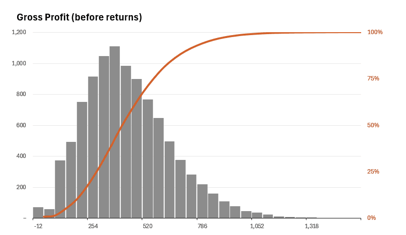
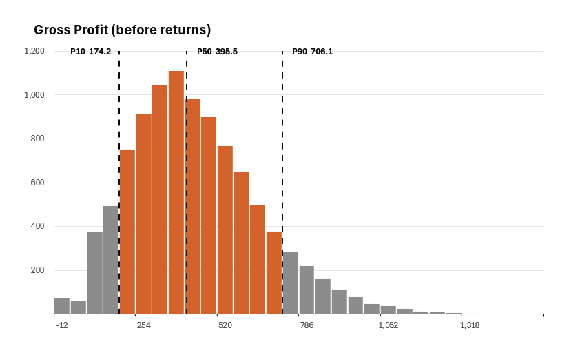
Two functions return the data behind the three charts every Monte Carlo report needs, each starting with a title row. fx.RiskChartHistλ puts everything a histogram needs into one spill — the title, the P10, P50 and P90 lines and the bins — so the lines can never drift from the bars they sit on. The bins are sized so that P10 and P90 fall exactly on bin edges, and the coloured band ends exactly at its lines.
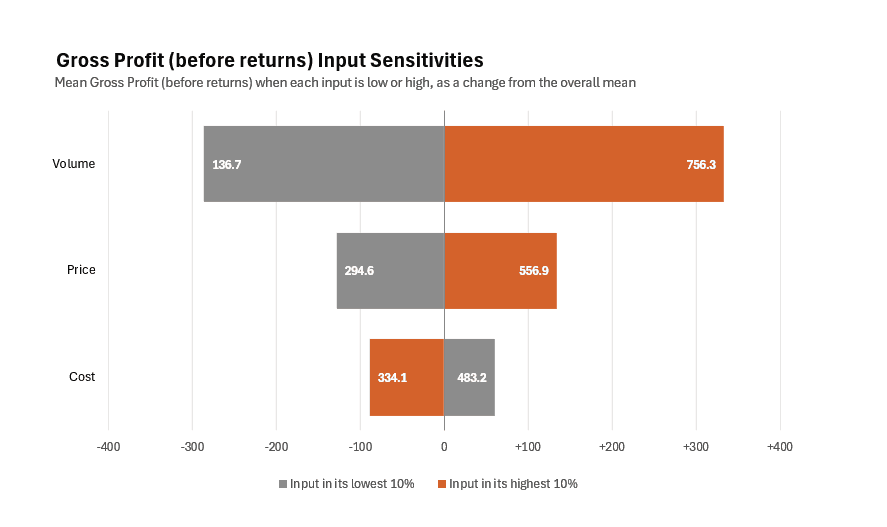
fx.RiskTornadoλ ranks the inputs by how far each one moves the output. By default it reports the output's mean when an input sits in its lowest 10% of trials and when it sits in its highest 10%, in the output's own units; the "rank" method reports each input's Spearman rank correlation instead.
XL Edge's Insert Monte Carlo Chart writes the data and draws a native Excel chart from it, with the title linked to the title row. Because the chart reads a live spill, it redraws when the model, the seed or the bin count changes. There is no picture to regenerate.
| Function | Arguments | Returns |
|---|---|---|
| fx.RiskChartHistλ | Trials, [Bins], [Lower], [Upper], [Name] | (Bins + 6) × 8, so 36 × 8 by default: the title, the Lower, P50 and Upper lines with their labels and positions, then one row per bin — centre, edges, in-band, tail and total counts, and cumulative %. |
| fx.RiskChartCDFλ | Trials, [Bins], [Points], [Lower], [Upper] | A smooth S-curve from P0 to P100 on the histogram's axis. Pass the histogram's Bins, Lower and Upper so the two share one grid. |
| fx.RiskTornadoλ | Output, Inputs, [Labels], [Method], [Tail], [Name] | A title row and subtitle, headers, then one row per input, largest effect first. Method "swing" (default) or "rank". |
| fx.RiskChartGridλ | Trials, Bins, Lower, Upper | The histogram's bin grid as {left edge, width}, used by the two chart functions above. |
| fx.RiskRankλ | Values | Average ranks, ties sharing the average of their positions. Sort-based, so it stays fast at 100,000 trials where RANK.AVG would not. |
Randomness
Two functions sit underneath all of the above. Most models never call them directly.
| Function | Arguments | Returns |
|---|---|---|
| fx.RiskUλ | Trials, [VarID], [Seed], [Method], [LHS] | A column of uniforms in (0, 1), the source for every distribution. Method is "HDR" (the default, reproducible) or "RAND" (volatile). LHS = TRUE switches on Latin hypercube stratification. An array passed as Trials is used directly as the uniforms, which is the hook for correlated sampling. |
| fx.RiskHDRλ | Counter, VarID, Entity, TimeID, AgentID | One HDR uniform, built from nested MOD arithmetic on fixed constants. Stateless: the same five inputs always return the same number, which is what makes every function above non-volatile. |
Building blocks
The distributions that Excel cannot invert directly are built on these. They are ordinary functions and can be called from a sheet, but most models will never need to.
| Function | Arguments | Returns |
|---|---|---|
| fx.RiskInvertλ | U, CDF, ToX, SLo, SHi, [Nodes], [Polish] | Numeric inversion of any continuous CDF passed in as a LAMBDA: one grid of Nodes points (default 4,096), monotone cubic interpolation on the normal-score scale, and optional Newton polishing. After Derflinger, Hörmann and Leydold (2010). The grid cost does not depend on the trial count. |
| fx.RiskDiscreteInvλ | U, Values, Cdf | Discrete sampling from a CDF table by binary search: the smallest value whose CDF is at least u. |
| fx.RiskHalfTInvλ | P, Q, DegFree | The quantile of |t|. Q is 1 − P, passed separately so the tails keep full precision. |
| fx.RiskInvGaussCDFλ | X, Mean, Shape | The inverse Gaussian CDF, combined in logs so it does not overflow. |
| fx.RiskNCBetaCDFλ | X, Shape1, Shape2, NonCentrality | The noncentral beta CDF, as a Poisson-weighted sum of BETA.DIST terms. Also used by the noncentral F. |
| fx.RiskNCStudentCDFλ | X, DegFree, NonCentrality | The noncentral t CDF, by Lenth's series (AS 243). |
| fx.RiskOwenTλ | H, A | Owen's T function, for the skew normal CDF: 20-point Gauss–Legendre quadrature, with Owen's identity for |A| > 1. |
Conventions worth checking
Argument conventions differ between Monte Carlo tools, and these get a wrong answer rather than an error, so they are stated plainly.
- Exponential takes the mean. fx.RiskExponλ(5) has a mean of 5. A tool that takes the rate reads the same 5 as a mean of 0.2.
- Lognormal takes log-scale parameters. Mean and StDev are those of ln(X) — @RISK's RiskLognorm2, not RiskLognorm.
- Weibull and Pareto take the shape first. Then the scale. For Pareto the scale is the minimum possible value — @RISK's RiskPareto, not RiskPareto2, which has them the other way round.
- Laplace and logistic take a scale, not the standard deviation. The Laplace sd is Scale × √2; the logistic sd is Scale × π / √3.
- Geometric and negative binomial count failures. From 0, as @RISK does — not tries from 1, as Excel's own functions and many statistics packages do. Add 1 to count the tries.
- Hypergeometric takes (Draws, Successes, Population). @RISK's (n, D, M). Other tools name and order the same three numbers differently.
- Skew normal's Location and Scale are not its mean and sd. They are only when Shape is 0.
- Give every input its own VarID. Two inputs sharing a VarID get the identical stream and move together perfectly — almost never what a model intends. XL Edge's selector assigns a fresh one each time.
- Inputs fed from a copula take no VarID of their own. The copula owns their randomness. Give the copula a VarID instead, and give two copulas in one model different ones, or they draw identical streams.
How it is checked
322 automated checks drive Excel directly, and all 322 pass. The HDR generator reproduces the self-check values published with the SIPmath standard to within 5 × 10⁻¹⁴, so it agrees with the reference implementations in other languages. Every closed-form distribution matches an independent reference inverse-CDF implementation fed the same uniforms, with a worst case of 3 × 10⁻¹², and every discrete distribution matches trial for trial. The five numerically inverted distributions are checked by a CDF round trip instead, because reference inverses are themselves unreliable far out in some tails: the worst relative error is about 10⁻⁸. The three risk measures match an independent implementation of the same estimators under both sign conventions.
Every copula matches an independent reference cell for cell, given the same uniforms; its Kendall's τ matches the closed form; every column passes a uniformity test; and Clayton shows its lower-tail and Gumbel its upper-tail dependence. The statistics blocks match an independent implementation on every row. Histogram counts tie to the trial count, the P-lines and S-curve equal independently computed percentiles, and tornado swings and rank correlations match independent calculations, including an input with tied values.
The rest cover monotonicity — a larger uniform never gives a smaller value, the property the copulas rely on — shape and moment tests at 20,000 trials, invalid-argument cases that must each return an error rather than a plausible wrong number, timing (the slowest distribution runs 100,000 trials in about a second), and a full recalculation plus a save, close and reopen, after which every value is identical and nothing shows #NAME?.
Attribution
Most of the mathematics here is textbook — the normal inverse, the exponential's −mean·ln(1 − u), the two-branch triangular quantile. What is borrowed is narrower, and it is credited here and inside the library itself.
- XLRisk (opens in a new tab) MIT licence. The original fifteen distributions — their catalogue, argument conventions and quantile expressions — the PERT reparameterisation and the Latin hypercube stratification all follow XLRisk.
- @RISK (Lumivero) Argument conventions for the distributions XLRisk does not have, followed so that existing models migrate by name.
- ProbabilityManagement.org (opens in a new tab) ChanceCalc Plus and PM_Lambda_functions, MIT licence, Copyright 2012–2026 Probability Management, Inc. The HDR generator formula, its constants and its five-slot seed scheme are theirs, and the Gaussian copula uses the Cholesky construction ChanceCalc Plus also uses. This library fixes a parameter-binding bug in their published HDR LAMBDA, which referenced timeId and agentId without declaring them.
- Hubbard Decision Research The HDR counter-based pseudo-random generator, published openly as part of the SIPmath standard.
- Tom Keelin The metalog distribution (Decision Analysis 13(4), 2016). Not built yet — credited because metalog support is on the roadmap.
- Published methods Numeric inversion after Derflinger, Hörmann and Leydold (ACM TOMACS 20(4), 2010); the noncentral t series of Lenth (Applied Statistics algorithm AS 243, 1989); Owen's T function (Owen, 1956); Expected Shortfall after Acerbi and Tasche (2002); the Archimedean copulas by frailty after Marshall and Olkin (1988) and Hofert (2008), with positive stable variates by Kanter's method (1975) and log-series variates by Kemp's LK algorithm (1981); and the t copula after McNeil, Frey and Embrechts, Quantitative Risk Management (2005).